Complexity

What is Complexity?

Complexity

In computer science, complexity refers to the performance characteristics of algorithms, such as
how much time or space they require to solve a problem. Complexity analysis helps in understanding
the efficiency of algorithms and predicting their behavior as the input size grows.

An algorithm’s performance isn’t measured by timing its execution on a specific machine, as this can
vary based on hardware and software configurations. Instead, complexity analysis focuses on the
algorithm’s behavior in terms of the input size, providing a more general understanding of its
efficiency.

Complexity is typically analyzed in terms of two main factors:

Time Complexity: The amount of time an algorithm takes to complete.
Space Complexity: The amount of memory an algorithm uses during execution.

Caption: Space and Time

Analyzing complexity enables us to evaluate the efficiency of an algorithm, compare different
approaches, and select the best solution for a given problem.

Big O Notation

What is Big O Notation?

Big O Notation is a mathematical representation used in computer science to describe the performance
or complexity of an algorithm. It focuses on the worst-case scenario, providing a measure of how an
algorithm’s execution time or space requirements grow relative to the size of its input.

In simple terms,

Big O helps us understand how an algorithm scales as the input size increases.

How Does Big O Work?

Big O abstracts away hardware, software, and other environmental factors, focusing solely on the
growth rate of an algorithm. It does not measure the exact runtime but categorizes algorithms based
on their performance trend as input size (‘n’) grows.

In Simple terms,

Big O tells us how an algorithm’s performance changes as the input size increases.

For example:

If an algorithm has a complexity of O(1), its runtime remains constant regardless of the input
size.
If an algorithm has a complexity of O(n), its runtime will grow linearly with the input size.
If an algorithm has a complexity of O(n²), its runtime will grow quadratically as the input
size increases.

How is Big O Calculated?

Big O is calculated by analyzing the most significant factors affecting an algorithm’s performance,
while ignoring constants and lower-order terms. Here are the steps to calculate it:

Identify the Input Size:
Determine the size of the input data, typically represented as ‘n’.
Analyze the Algorithm:
Break down the algorithm into steps and determine how many operations are performed relative to
‘n’.
Focus on the Dominant Term:
Identify the term with the highest growth rate as ‘n’ increases. Ignore constants and smaller
terms, as they have a negligible effect on large input sizes.

Example:

fun sum(numbers: List<Int>): Int {
    var total = 0
    for (num in numbers) { // O(n)
        total += num
    }
    return total
}

Here, the loop runs ‘n’ times, so the time complexity is O(n).

Getting over your head? Don’t worry!
Let’s use a real-world scenario to understand this better: making a cup of tea.

Imagine the steps to make tea:
Boil water.
Add tea leaves or a tea bag.
Add sugar (let’s assume you add sugar one spoon at a time).
Stir the tea.
Pour into a cup.

Now, let’s focus on the sugar step. If you decided to add 2 spoons of sugar, this step would take 2
operations because you add sugar twice.
If you want 3 spoons of sugar, it would take 3 operations, and so on. If you decide to add n
spoons of sugar, this step would take n operations because each spoon of sugar requires a
separate action. The complexity of this step depends on the number of spoons of sugar you want to
add, making it O(n).

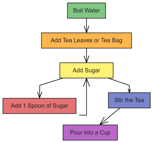
Caption: Tea Making Flow

Here’s a breakdown of the entire process and its time complexity:

Boiling water: This takes a fixed amount of time, no matter how much tea you make. O(1).
Adding tea leaves or a tea bag: Again, this is a single action, so it’s O(1).
Adding sugar: This depends on the number of spoons, so it’s O(n).
Stirring the tea: This is a single action, so it’s O(1).
Pouring into a cup: Another single action, making it O(1).

When we combine the steps, the overall complexity is determined by the step with the highest growth
rate. In this case, the O(n) step (adding sugar) dominates because it depends on the variable *
n*, while the other steps remain constant. Therefore, the time complexity for making tea in this
example is O(n).

Time Complexity

What is Time Complexity?

Time complexity refers to the amount of time an algorithm takes to complete, expressed as a function
of the input size (‘n’). It provides an estimate of how an algorithm’s runtime will grow as the size
of the input increases.

In other words,

Time complexity measures the efficiency of an algorithm in terms of time as the input size grows.

Analyzing time complexity helps developers compare different algorithms and choose the one that
performs best for their specific use case.

Common Time Complexities

Below are some common time complexities, their explanations, and examples:

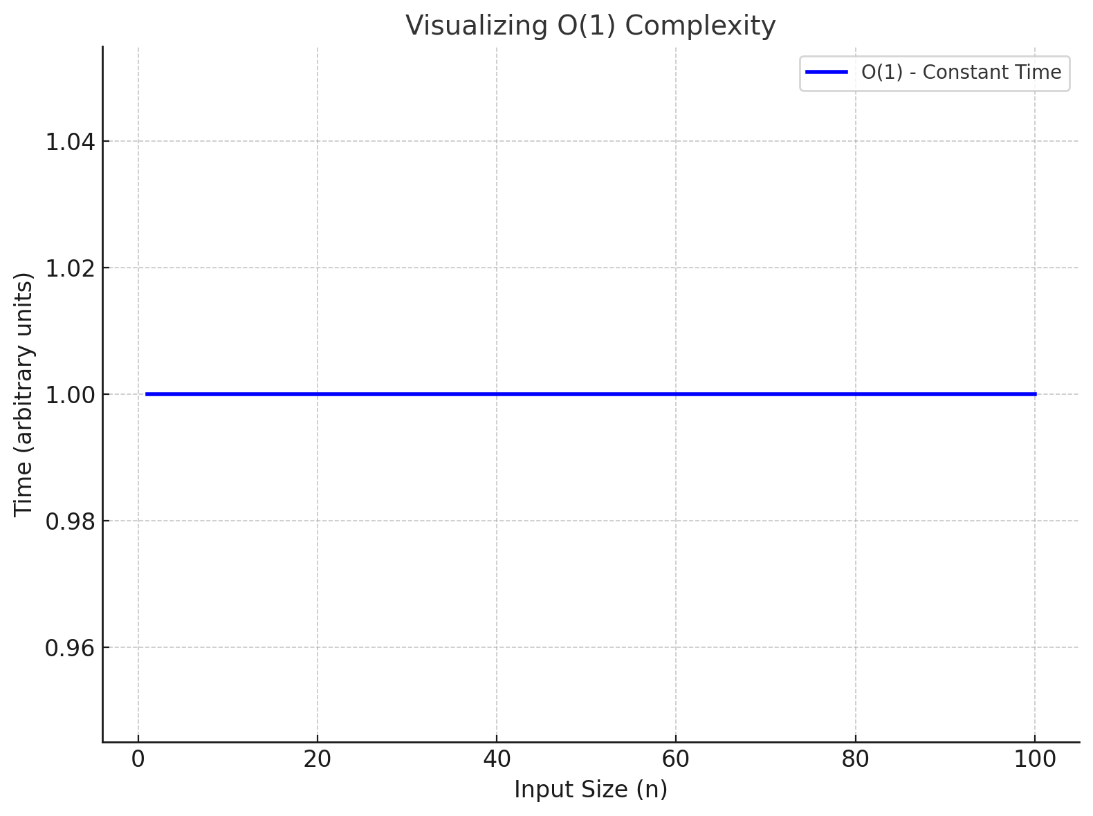
1. O(1) - Constant Time

The algorithm’s runtime remains constant, regardless of the input size.

In Real-world scenarios, like our tea-making example:

Boiling water: This step takes a fixed amount of time, no matter how much tea you make.
Adding tea leaves or a tea bag: This is a single action, so it’s constant.

These steps have a time complexity of O(1). Because they take the same amount of time,
regardless of the input size.

Example:

fun getFirstElement(numbers: List<Int>): Int {
    return numbers[0] // Always one operation
}

O of 1
O(1)

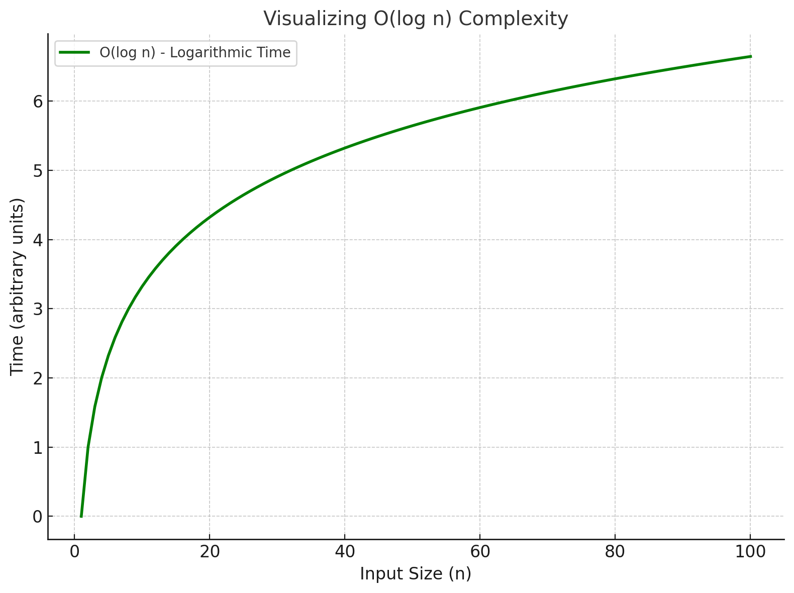
2. O(log n) - Logarithmic Time

The runtime grows logarithmically, often occurring when the input size is reduced by half at each
step.

In Real-world scenarios, like searching for a name in a phone book:

If you start searching in the middle, you can eliminate half the book.
Then, you can eliminate half of the remaining half, and so on.
This process reduces the search space by half at each step.

In this case, the time complexity is O(log n), because the search time grows logarithmically as
the input size increases.

Example:

fun binarySearch(numbers: List<Int>, target: Int): Boolean {
    var low = 0
    var high = numbers.size - 1
    while (low <= high) {
        val mid = (low + high) / 2
        when {
            numbers[mid] == target -> return true
            numbers[mid] < target -> low = mid + 1
            else -> high = mid - 1
        }
    }
    return false
}

O of log n
O(log n)

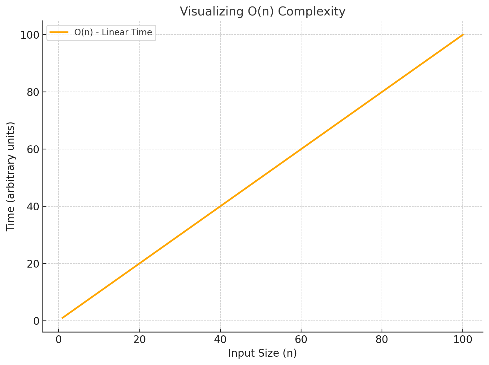
3. O(n) - Linear Time

The runtime grows linearly with the input size.

In Real-world scenarios, like counting the number of books on a shelf:

If you have 10 books, you count each one.
If you have 100 books, you count each one.

This process scales linearly with the number of books, making it O(n), where ‘n’ is the number
of books.

Example:

fun sum(numbers: List<Int>): Int {
    var total = 0
    for (num in numbers) {
        total += num
    }
    return total
}

O of n
O(n)

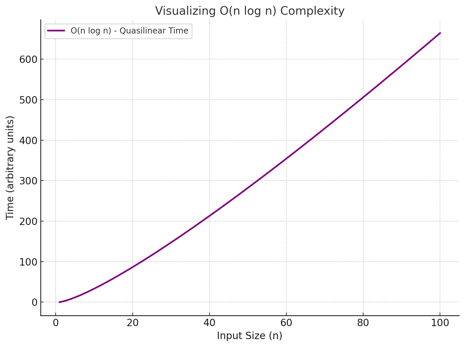
4. O(n log n) - Linearithmic Time

The runtime grows proportionally to n times the logarithm of n, often found in efficient sorting
algorithms.

In Real-world scenarios, like sorting a deck of cards:

If you use a sorting algorithm like Merge Sort or Quick Sort, the time complexity is O(n log
n).
These algorithms divide the deck into smaller parts, sort them, and then merge them back
together.
The time taken grows linearly with the number of cards, but also scales logarithmically due to
the divide-and-conquer approach.

Example:

fun mergeSort(numbers: List<Int>): List<Int> {
    if (numbers.size <= 1) return numbers
    val mid = numbers.size / 2
    val left = mergeSort(numbers.subList(0, mid))
    val right = mergeSort(numbers.subList(mid, numbers.size))
    return merge(left, right)
}

fun merge(left: List<Int>, right: List<Int>): List<Int> {
    var result = mutableListOf<Int>()
    var i = 0
    var j = 0
    while (i < left.size && j < right.size) {
        if (left[i] <= right[j]) {
            result.add(left[i++])
        } else {
            result.add(right[j++])
        }
    }
    result.addAll(left.subList(i, left.size))
    result.addAll(right.subList(j, right.size))
    return result
}

O of n log n

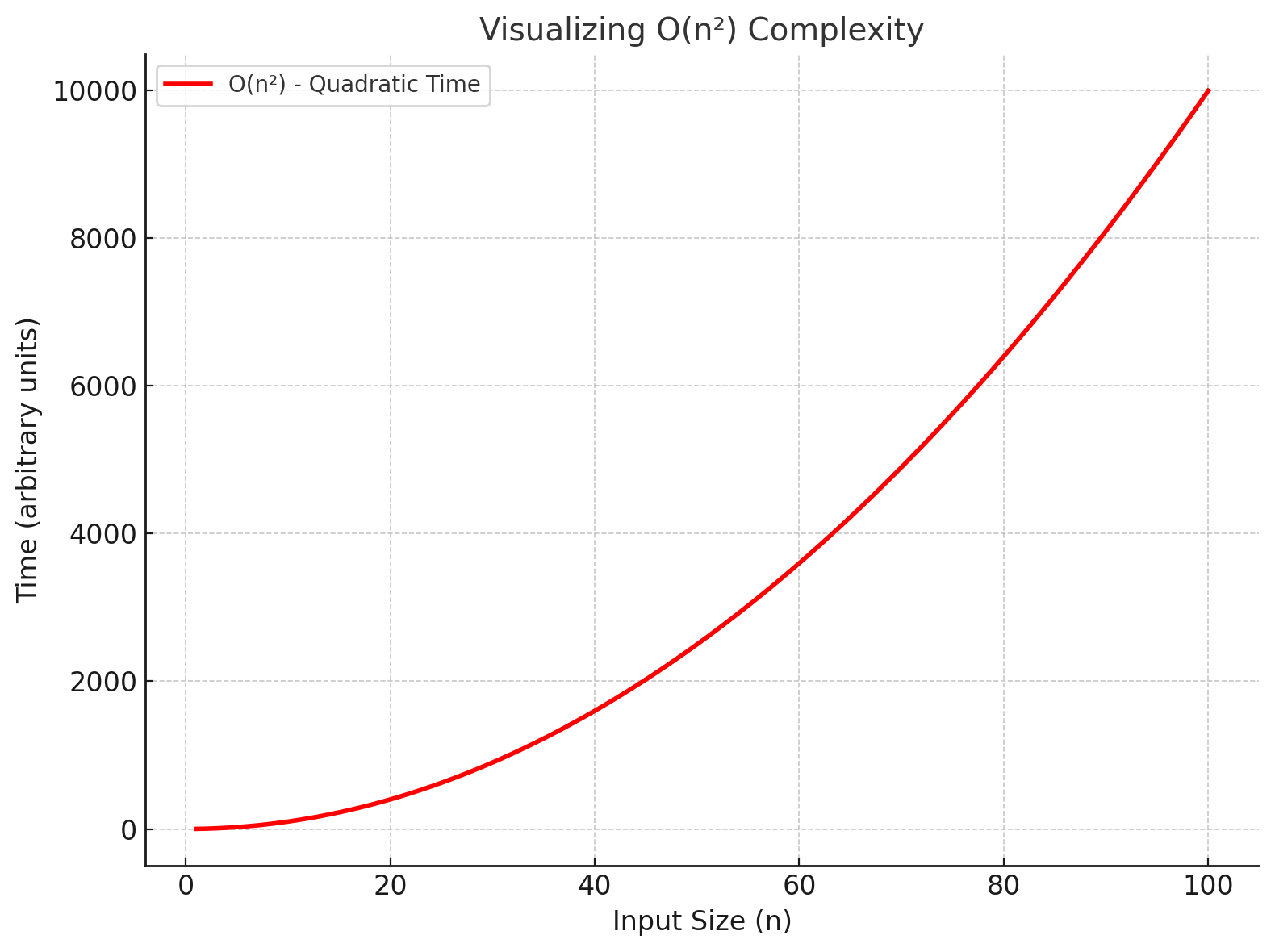
5. O(n²) - Quadratic Time

The runtime grows quadratically, often found in nested loops.

In Real-world scenarios, like comparing one book to every other book on a shelf:

If you have 10 books, you compare each book to the other 9.
If you have 100 books, you compare each book to the other 99.

This process scales quadratically with the number of books, making it O(n²).

Example:

fun findPairs(numbers: List<Int>) {
    for (i in numbers.indices) {
        for (j in i + 1 until numbers.size) {
            println("Pair: ${numbers[i]}, ${numbers[j]}")
        }
    }
}

O of n²

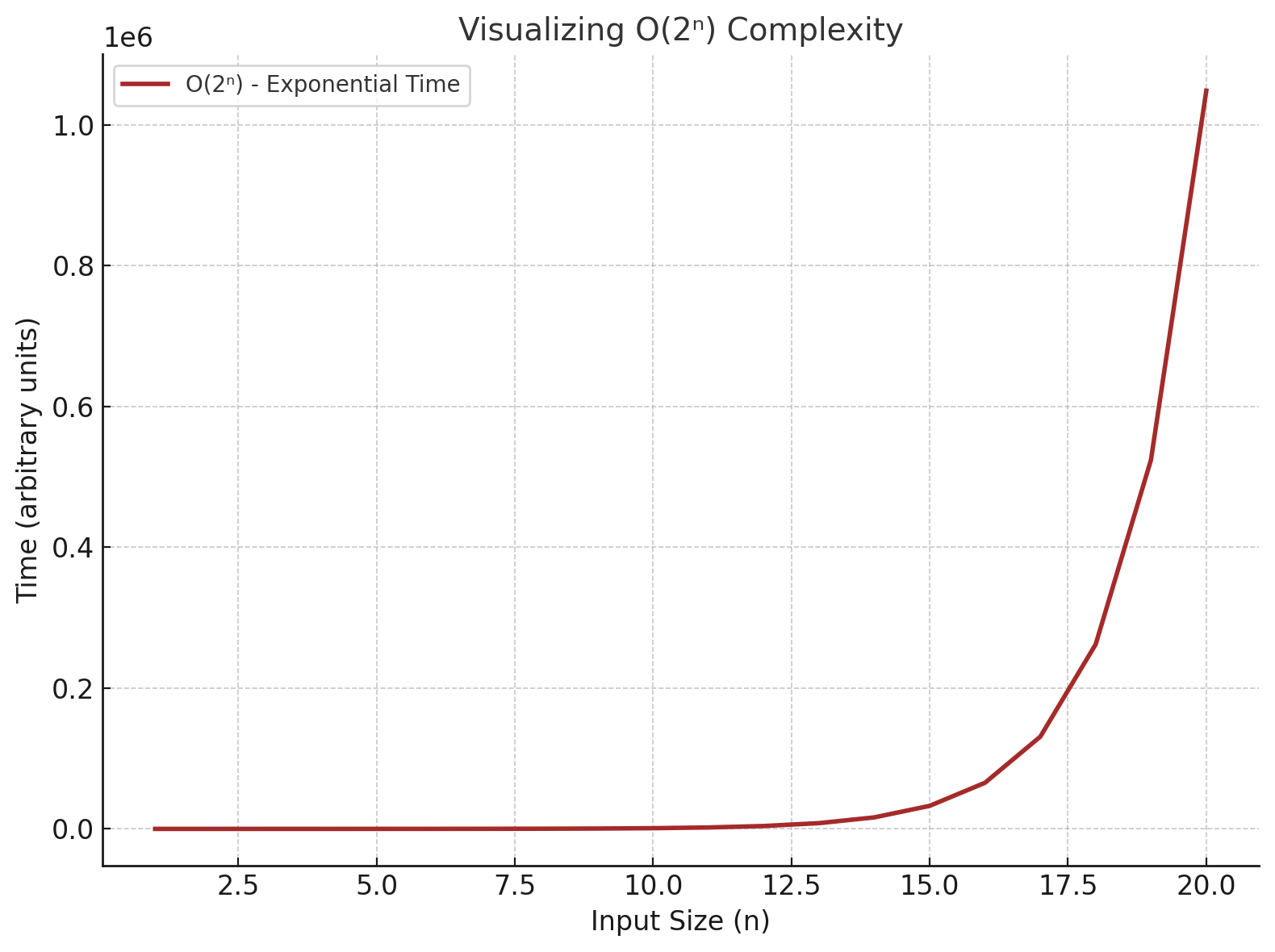
6. O(2ⁿ) - Exponential Time

The runtime doubles with each additional input, often found in algorithms exploring all
possibilities.

In Real-world scenarios, like solving the Tower of Hanoi puzzle:

If you have 1 disk, it takes 2 steps.
If you have 2 disks, it takes 4 steps.
If you have 3 disks, it takes 8 steps.

This process scales exponentially with the number of disks, making it O(2ⁿ).

Example:

fun fibonacci(n: Int): Int {
    if (n <= 1) return n
    return fibonacci(n - 1) + fibonacci(n - 2)
}

O of 2ⁿ

Why Time Complexity Matters

Performance Analysis: Helps in comparing algorithms and selecting the most efficient one.
Scalability: Algorithms with lower time complexity handle larger datasets more effectively.
Resource Management: Ensures that algorithms run within time constraints, especially in
real-time systems.
Optimization: Identifies bottlenecks and areas for improvement in algorithms.
Predictability: Provides insights into how an algorithm will perform as the input size grows.

Now that we’ve explored how algorithms perform in terms of time, let’s look at how they manage
memory resources with Space Complexity.

Space Complexity

What is Space Complexity?

Space complexity refers to the amount of memory an algorithm uses as a function of the input size (
‘n’). It helps us understand how efficiently an algorithm utilizes memory resources, encompassing
both fixed and dynamic memory usage.

In other words:

Space complexity measures how the memory usage of an algorithm grows with the size of the input.

Analyzing space complexity ensures that algorithms run within the memory constraints of a system,
which is especially critical for environments like embedded systems or mobile devices.

Components of Space Complexity

Fixed Space Requirements:
- Memory allocated for constants, variables, and temporary storage.
- This memory does not depend on the size of the input.
- Example: Storing a few fixed variables in an algorithm (e.g., counters, pointers).
Dynamic Space Requirements:
- Memory required for dynamic data structures like arrays, recursion stacks, or heap
  allocations.
- This memory grows with the input size.
- Example: Recursion depth or the size of an input array.

Common Space Complexities

O(1) - Constant Space

The algorithm uses a fixed amount of memory regardless of the input size.

In real-life scenarios,

This is like writing down the first page of a book’s index on a sticky note—you store only one
page regardless of the book’s size.

Example:

fun sum(numbers: List<Int>): Int {
    var total = 0
    for (num in numbers) {
        total += num
    }
    return total
}

O(n) - Linear Space

Memory usage grows linearly with the input size.

In real-life scenarios,

Storing every book title on a shelf in separate sticky notes—if there are 100 books, you’ll
need 100 sticky notes.

Example:

fun copyArray(numbers: List<Int>): List<Int> {
    val newNumbers = mutableListOf<Int>() // Space grows with input size
    for (num in numbers) {
        newNumbers.add(num)
    }
    return newNumbers
}

O(log n) - Logarithmic Space

Memory usage grows logarithmically, often in divide-and-conquer algorithms.

In real-life scenarios,

Searching for a name in a sorted phone book and writing down only the range of pages you’re
currently searching through.

Example:

fun binarySearchRecursive(numbers: List<Int>, target: Int, low: Int, high: Int): Boolean {
    if (low > high) return false
    val mid = (low + high) / 2
    return when {
        numbers[mid] == target -> true
        numbers[mid] < target -> binarySearchRecursive(numbers, target, mid + 1, high)
        else -> binarySearchRecursive(numbers, target, low, mid - 1)
    }
}

O(n²) - Quadratic Space

Memory usage grows quadratically with input size, often in algorithms involving 2D matrices.

In real-life scenarios,

Writing down all possible pairings of books on a shelf—if there are 10 books, you’ll write down
100 pairs.

Example:

fun createMatrix(n: Int): Array<Array<Int>> {
    val matrix = Array(n) { Array(n) { 0 } } // Creates n x n matrix
    return matrix
}

O(2ⁿ) - Exponential Space

Memory usage doubles with each additional input, often in algorithms exploring all subsets or
combinations.

In real-life scenarios,

Listing all possible outfits from a wardrobe with 10 items—each item doubles the combinations.

Programming Example:

fun fibonacciRecursive(n: Int): Int {
    if (n <= 1) return n
    return fibonacciRecursive(n - 1) + fibonacciRecursive(n - 2)
}

Why Space Complexity Matters

Memory is Finite: Critical in memory-constrained environments like embedded systems and
mobile devices.
Performance Impact: Excessive memory usage can lead to slower programs or crashes.
Scalability: Algorithms with lower space complexity handle larger datasets more effectively.
Balanced Trade-offs: Choosing the right algorithm involves trade-offs between time and space
complexity.

Conclusion

Understanding complexity is essential for writing efficient algorithms that scale with input size.
Time complexity helps in analyzing an algorithm’s runtime behavior, while space complexity focuses
on
its memory usage. By analyzing these factors, developers can optimize algorithms, predict their
performance, and make informed decisions when selecting the best solution for a given problem.

What is Complexity?

Big O Notation

What is Big O Notation?

How Does Big O Work?

How is Big O Calculated?

Time Complexity

What is Time Complexity?

Common Time Complexities

1. O(1) - Constant Time

2. O(log n) - Logarithmic Time

3. O(n) - Linear Time

4. O(n log n) - Linearithmic Time

5. O(n²) - Quadratic Time

6. O(2ⁿ) - Exponential Time

Why Time Complexity Matters

Space Complexity

What is Space Complexity?

Components of Space Complexity

Common Space Complexities

Why Space Complexity Matters

Conclusion

References

Me